Webinar notebook#
%matplotlib inline
import logging
from warnings import filterwarnings
from aesara import pprint
from matplotlib import pyplot as plt, ticker
import numpy as np
import pandas as pd
import scipy as sp
import seaborn as sns
from sklearn.preprocessing import StandardScaler
import xarray as xr
filterwarnings(
    'ignore', category=UserWarning, module='pymc',
    message="Unable to validate shapes: Cannot sample from flat variable",
)
filterwarnings('ignore', category=RuntimeWarning, module='pymc')
def filter_metropolis(record):
    return not (record.msg.startswith(">Metropolis") or record.msg == "CompoundStep")

logging.getLogger('pymc').addFilter(filter_metropolis)
# configure pyplot for readability when rendered as a slideshow and projected
FIG_WIDTH, FIG_HEIGHT = 8, 6
plt.rc('figure', figsize=(FIG_WIDTH, FIG_HEIGHT))

LABELSIZE = 14
plt.rc('axes', labelsize=LABELSIZE)
plt.rc('axes', titlesize=LABELSIZE)
plt.rc('figure', titlesize=LABELSIZE)
plt.rc('legend', fontsize=LABELSIZE)
plt.rc('xtick', labelsize=LABELSIZE)
plt.rc('ytick', labelsize=LABELSIZE)

dollar_formatter = ticker.StrMethodFormatter("${x:,.0f}")
pct_formatter = ticker.StrMethodFormatter("{x:.1%}")

sns.set(color_codes=True)

About this talk#
Agenda#
Probabilistic programming from two perspectives
Philosophical: storytelling with data
Mathematical: Monte Carlo methods
Probabilistic programming with PyMC
The Monty Hall problem
Robust regression
Hamiltonian Monte Carlo
Aesara
Lego? example
Next Steps
All the code that is shown in this webinar can be executed from its website. Therefore you have two ways to follow along:
Click on the run code button and execute the code straight from this page
Clone the GitHub repo: pymc-devs/pymc-data-umbrella and follow along locally using Jupyter
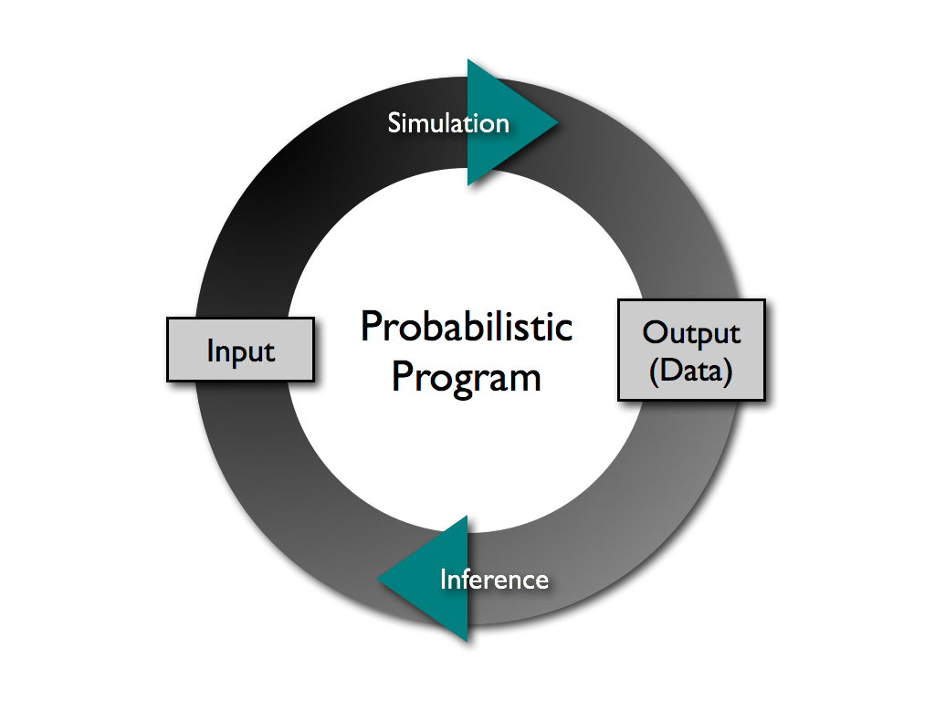
Probabilistic programming from two perspectives#
Philosophical#
(Classical) Data science —— inference enables story telling#
Probabilistic programming —— story telling enables inference#
Bayesian inference —— quantifying uncertainty#

Mathematical#
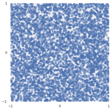
Monte Carlo methods#
SEED = 123456789 # for reproducibility
rng = np.random.default_rng(SEED)
N = 5_000
x, y = rng.uniform(-1, 1, size=(2, N))
fig, ax = plt.subplots(subplot_kw={"aspect": "equal"})

ax.scatter(x, y, alpha=0.5);

ax.set_xticks([-1, 0, 1]);
ax.set_xlim(-1.01, 1.01);

ax.set_yticks([-1, 0, 1]);
ax.set_ylim(-1.01, 1.01);
fig
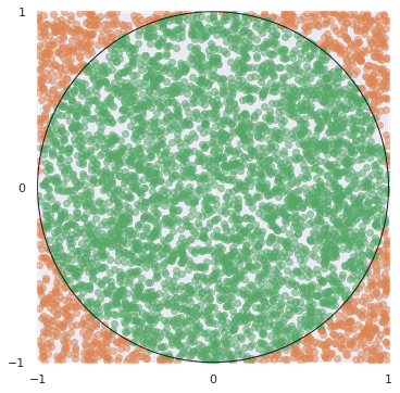
in_circle = x**2 + y**2 < 1
fig, ax = plt.subplots(subplot_kw={"aspect": "equal"})

ax.scatter(x[~in_circle], y[~in_circle],
           c='C1', alpha=0.5);
ax.scatter(x[in_circle], y[in_circle],
           c='C2', alpha=0.5);

ax.add_artist(plt.Circle((0, 0), 1, fill=False, edgecolor='k'));

ax.set_xticks([-1, 0, 1]);
ax.set_xlim(-1.01, 1.01);

ax.set_yticks([-1, 0, 1]);
ax.set_ylim(-1.01, 1.01);
fig
4 * in_circle.sum() / N
3.1488
Monte Carlo methods —— approximating (intractible) integrals#
fig, ax = plt.subplots(subplot_kw={"aspect": "equal"})

ax.set_facecolor('C1');
ax.add_artist(plt.Circle((0, 0), 1, facecolor='C2', edgecolor='k'));
ax.plot([0, 0, 1], [1, 0, 0], c='k');

ax.set_xticks([-1, 0, 1]);
ax.set_xlim(-1.01, 1.01);

ax.set_yticks([-1, 0, 1]);
ax.set_ylim(-1.01, 1.01);
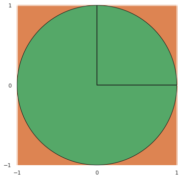
fig
Bayes’ Theorem —— (often) intractible integrals#
Forcing this term to be analytically tractible drastically limits the richness of the models we can consider.
Probabilistic Programming with PyMC#
The Monty Hall Problem#

Mathematical solution#
PyMC solution#
Initially, we have no information about which door the prize is behind.
import pymc as pm

with pm.Model() as monty_model:
    prize = pm.DiscreteUniform("prize", 0, 2, initval=0)
If we choose the first door:
| Prize behind | Door 1 | Door 2 | Door 3 |
|---|---|---|---|
| Door 1 | No | Yes | Yes |
| Door 2 | No | No | Yes |
| Door 3 | No | Yes | No |
from aesara import tensor as aet
p_open = aet.switch(
    aet.eq(prize, 0),
    np.array([0, 0.5, 0.5]), # it is behind the first door
    aet.switch(
        aet.eq(prize, 1),
        np.array([0, 0, 1]), # it is behind the second door
        np.array([0, 1, 0])  # it is behind the third door
    )
)
Monty opened the third door, revealing a goat.
with monty_model:
    opened = pm.Categorical("opened", p_open, observed=2)
with monty_model:
    monty_trace = pm.sample(10_000)
/home/oriol/miniconda3/envs/arviz/lib/python3.9/site-packages/pymc/model.py:984: FutureWarning: `Model.initial_point` has been deprecated. Use `Model.recompute_initial_point(seed=None)`.
  warnings.warn(
Multiprocess sampling (4 chains in 4 jobs)
Metropolis: [prize]
/home/oriol/miniconda3/envs/arviz/lib/python3.9/site-packages/pymc/model.py:984: FutureWarning: `Model.initial_point` has been deprecated. Use `Model.recompute_initial_point(seed=None)`.
  warnings.warn(
Sampling 4 chains for 1_000 tune and 10_000 draw iterations (4_000 + 40_000 draws total) took 8 seconds.
The number of effective samples is smaller than 25% for some parameters.
print(monty_trace.posterior["prize"])
<xarray.DataArray 'prize' (chain: 4, draw: 10000)>
array([[0, 0, 0, ..., 0, 0, 0],
       [1, 1, 1, ..., 0, 1, 1],
       [1, 1, 1, ..., 1, 1, 1],
       [1, 1, 1, ..., 0, 1, 1]])
Coordinates:
  * chain    (chain) int64 0 1 2 3
  * draw     (draw) int64 0 1 2 3 4 5 6 7 ... 9993 9994 9995 9996 9997 9998 9999
print((monty_trace.posterior["prize"] == 0).mean())
<xarray.DataArray 'prize' ()>
array(0.33255)
fig, ax = plt.subplots()

monty_trace.posterior["prize"].plot.hist(ax=ax, bins=[-.5, .5, 1.5], density=True)

ax.set_xticks([0, 1]);
ax.set_xlabel("Door");

ax.yaxis.set_major_formatter(pct_formatter);
ax.set_yticks(np.linspace(0, 1, 5));
ax.set_ylabel("Proability prize is behind door");
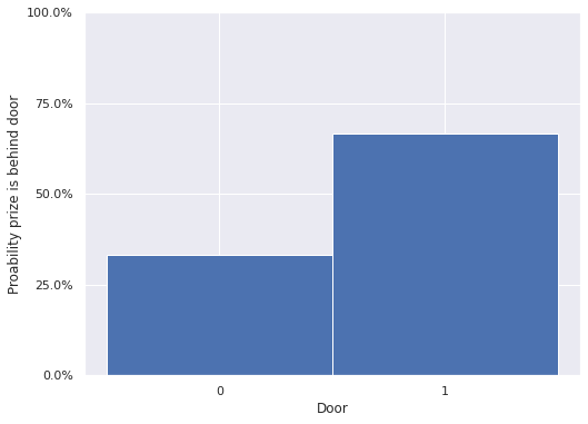
fig
Two key components#
PyMC distributions#

|

|

|
|
|
|
Aesara is a Python library that allows you to define, optimize, and evaluate mathematical expressions involving multi-dimensional arrays efficiently. Aesara features:
Tight integration with NumPy – Use numpy.ndarray in Aesara-compiled functions.
Efficient symbolic differentiation – Aesara does your derivatives for functions with one or many inputs.
Speed and stability optimizations – Get the right answer for log(1+x) even when x is really tiny.
Dynamic C/JAX/Numba code generation – Evaluate expressions faster.
Aesara is based on Theano, which has been powering large-scale computationally intensive scientific investigations since 2007.
Robust Regression#
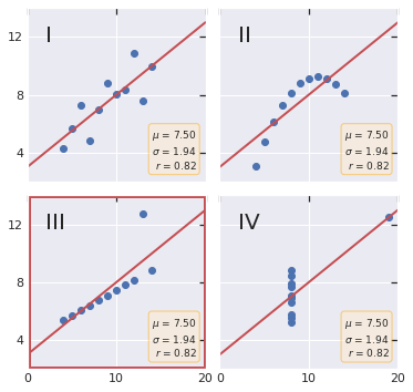
Anscombe’s quartet#
This code for plotting Anscombe’s quartet is adapted from the matplotlib documentation.
x = np.array([10, 8, 13, 9, 11, 14, 6, 4, 12, 7, 5], dtype=np.float64)
y1 = np.array([8.04, 6.95, 7.58, 8.81, 8.33, 9.96, 7.24, 4.26, 10.84, 4.82, 5.68])
y2 = np.array([9.14, 8.14, 8.74, 8.77, 9.26, 8.10, 6.13, 3.10, 9.13, 7.26, 4.74])
y3 = np.array([7.46, 6.77, 12.74, 7.11, 7.81, 8.84, 6.08, 5.39, 8.15, 6.42, 5.73])
x4 = np.array([8, 8, 8, 8, 8, 8, 8, 19, 8, 8, 8])
y4 = np.array([6.58, 5.76, 7.71, 8.84, 8.47, 7.04, 5.25, 12.50, 5.56, 7.91, 6.89])

datasets = {
    'I': (x, y1),
    'II': (x, y2),
    'III': (x, y3),
    'IV': (x4, y4)
}

fig, axs = plt.subplots(2, 2, sharex=True, sharey=True, figsize=(6, 6),
                        gridspec_kw={'wspace': 0.08, 'hspace': 0.08})
axs[0, 0].set(xlim=(0, 20), ylim=(2, 14))
axs[0, 0].set(xticks=(0, 10, 20), yticks=(4, 8, 12))

for ax, (label, (x_, y)) in zip(axs.flat, datasets.items()):
    ax.text(0.1, 0.9, label, fontsize=20, transform=ax.transAxes, va='top')
    ax.tick_params(direction='in', top=True, right=True)
    ax.plot(x_, y, 'o')

    # linear regression
    p1, p0 = np.polyfit(x_, y, deg=1)  # slope, intercept
    ax.axline(xy1=(0, p0), slope=p1, color='r', lw=2)

    # add text box for the statistics
    stats = (f'$\\mu$ = {np.mean(y):.2f}\n'
             f'$\\sigma$ = {np.std(y):.2f}\n'
             f'$r$ = {np.corrcoef(x_, y)[0][1]:.2f}')
    bbox = dict(boxstyle='round', fc='blanchedalmond', ec='orange', alpha=0.5)
    ax.text(0.95, 0.07, stats, fontsize=9, bbox=bbox,
            transform=ax.transAxes, horizontalalignment='right')

axs[1, 0].add_artist(plt.Rectangle((0, 2), 20, 12, fill=False, edgecolor='r', lw=5));
fig
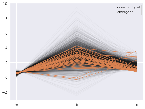
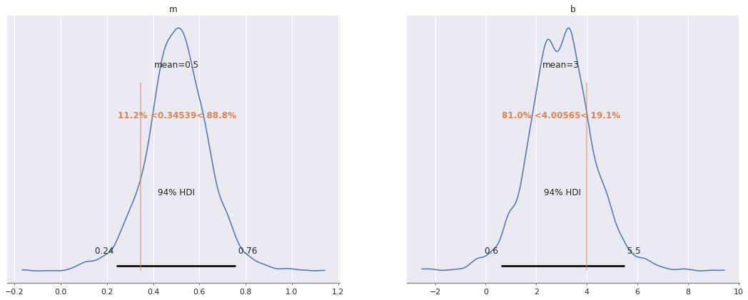
Ordinary least squares#
Assumption: All values of \(m, b \in \mathbb{R}\), \(\sigma > 0\) are equally likely
with pm.Model() as ols_model:
    m = pm.Flat("m")
    b = pm.Flat("b")

    σ = pm.HalfFlat("σ")
This is equivalent to
with ols_model:
    y_obs = pm.Normal("y_obs", m * x + b, σ, observed=y3)
with ols_model:
    ols_trace = pm.sample()
Auto-assigning NUTS sampler...
Initializing NUTS using jitter+adapt_diag...
/home/oriol/miniconda3/envs/arviz/lib/python3.9/site-packages/pymc/model.py:984: FutureWarning: `Model.initial_point` has been deprecated. Use `Model.recompute_initial_point(seed=None)`.
  warnings.warn(
Multiprocess sampling (4 chains in 4 jobs)
NUTS: [m, b, σ]
Sampling 4 chains for 1_000 tune and 1_000 draw iterations (4_000 + 4_000 draws total) took 7 seconds.
There were 2 divergences after tuning. Increase `target_accept` or reparameterize.
There were 47 divergences after tuning. Increase `target_accept` or reparameterize.
The acceptance probability does not match the target. It is 0.6208, but should be close to 0.8. Try to increase the number of tuning steps.
There were 8 divergences after tuning. Increase `target_accept` or reparameterize.
There were 6 divergences after tuning. Increase `target_accept` or reparameterize.
The estimated number of effective samples is smaller than 200 for some parameters.
import arviz as az
az.plot_parallel(ols_trace);
Two more key components#
ArviZ is a Python package for exploratory analysis of Bayesian models. Includes functions for posterior analysis, data storage, sample diagnostics, model checking, and comparison.
The goal is to provide backend-agnostic tools for diagnostics and visualizations of Bayesian inference in Python, by first converting inference data into xarray objects. See here for more on xarray and ArviZ usage and here for more on InferenceData structure and specification.
type(ols_trace)
arviz.data.inference_data.InferenceData
type(ols_trace.posterior)
xarray.core.dataset.Dataset
xarray (formerly xray) is an open source project and Python package that makes working with labelled multi-dimensional arrays simple, efficient, and fun!
Xarray is inspired by and borrows heavily from pandas, the popular data analysis package focused on labelled tabular data. It is particularly tailored to working with netCDF files, which were the source of xarray’s data model, and integrates tightly with dask for parallel computing.
m_robust, b_robust = np.polyfit(x[x != 13], y3[x != 13], deg=1)

az.plot_posterior(ols_trace, var_names=["m", "b"],
                  ref_val=[m_robust, b_robust]);
REG_THIN = 5
thin_slice = slice(None, None, REG_THIN)
xr_plot = xr.DataArray(np.linspace(-1,15), dims="plot")
fig, ax = plt.subplots()

thinned = ols_trace.posterior.stack(sample=("chain", "draw")).isel(sample=thin_slice)
ax.plot(xr_plot, xr_plot*thinned.m + thinned.b, c="C0", alpha=0.025)

ax.scatter(x, y3);

ax.axline(xy1=(0, p0), slope=p1,
          color='r', ls='--', zorder=5,
          label="NumPy OLS");

ax.axline(
    (0, ols_trace.posterior["b"].mean()),
    slope=ols_trace.posterior["m"].mean(),
    c='C0', label="PyMC OLS"
);

ax.set(xlim=(-1, 15), ylim=(-2, 14));
ax.legend();
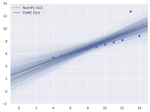
fig
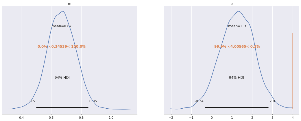
Ridge regression#
Ridge regression is equivalent to normal priors on \(m\) and \(b\).
with pm.Model() as ridge_model:
    m = pm.Normal("m", 0., 1)
    b = pm.Normal("b", 0., 1)

    σ = pm.HalfNormal("σ", 1)
    y_obs = pm.Normal("y_obs", m * x + b, σ, observed=y3)

    ridge_trace = pm.sample()
Auto-assigning NUTS sampler...
Initializing NUTS using jitter+adapt_diag...
/home/oriol/miniconda3/envs/arviz/lib/python3.9/site-packages/pymc/model.py:984: FutureWarning: `Model.initial_point` has been deprecated. Use `Model.recompute_initial_point(seed=None)`.
  warnings.warn(
Multiprocess sampling (4 chains in 4 jobs)
NUTS: [m, b, σ]
Sampling 4 chains for 1_000 tune and 1_000 draw iterations (4_000 + 4_000 draws total) took 7 seconds.
There were 5 divergences after tuning. Increase `target_accept` or reparameterize.
There were 2 divergences after tuning. Increase `target_accept` or reparameterize.
az.plot_posterior(ridge_trace, var_names=["m", "b"],
                  ref_val=[m_robust, b_robust]);
fig, ax = plt.subplots()

thinned = ridge_trace.posterior.stack(sample=("chain", "draw")).isel(sample=thin_slice)
ax.plot(xr_plot, xr_plot*thinned.m + thinned.b, c="C1", alpha=0.025)

ax.scatter(x, y3);

ax.axline(xy1=(0, p0), slope=p1,
          color='r', ls='--', zorder=5,
          label="NumPy OLS");

ax.axline(
    (0, ols_trace.posterior["b"].mean()),
    slope=ols_trace.posterior["m"].mean(),
    c='C0', label="PyMC OLS"
);
ax.axline(
    (0, ridge_trace.posterior["b"].mean()),
    slope=ridge_trace.posterior["m"].mean(),
    c='C1', label="PyMC Ridge"
);

ax.set(xlim=(-1, 15), ylim=(-2, 14));
ax.legend();
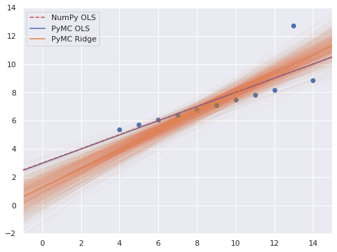
fig
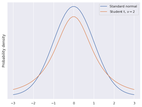
Robust regression#
Student’s t-distribution has fatter tails than the normal distribution.
fig, ax = plt.subplots()

x_plot = np.linspace(-3, 3)
ax.plot(x_plot, sp.stats.norm.pdf(x_plot),
        label="Standard normal");

DF = 2
ax.plot(x_plot, sp.stats.t.pdf(x_plot, DF),
        label=f"Student t, $\\nu = {DF}$");

ax.set_yticks([]);
ax.set_ylabel("Probability density");

ax.legend();
fig
with pm.Model() as robust_model:
    m = pm.Normal("m", 0., 1)
    b = pm.Normal("b", 0., 1)

    σ = pm.HalfNormal("σ", 1)
A Student t-likelihood is less sensitive to outliers
with robust_model:
    ν = pm.Uniform("ν", 1, 10, initval=3)
    y_obs = pm.StudentT(
        "y_obs",
        nu=ν, mu=m * x + b, sigma=σ,
        observed=y3
    )

    robust_trace = pm.sample()
Auto-assigning NUTS sampler...
Initializing NUTS using jitter+adapt_diag...
/home/oriol/miniconda3/envs/arviz/lib/python3.9/site-packages/pymc/model.py:984: FutureWarning: `Model.initial_point` has been deprecated. Use `Model.recompute_initial_point(seed=None)`.
  warnings.warn(
Multiprocess sampling (4 chains in 4 jobs)
NUTS: [m, b, σ, ν]
/home/oriol/miniconda3/envs/arviz/lib/python3.9/site-packages/pymc/model.py:984: FutureWarning: `Model.initial_point` has been deprecated. Use `Model.recompute_initial_point(seed=None)`.
  warnings.warn(
Sampling 4 chains for 1_000 tune and 1_000 draw iterations (4_000 + 4_000 draws total) took 17 seconds.
The acceptance probability does not match the target. It is 0.6952, but should be close to 0.8. Try to increase the number of tuning steps.
The number of effective samples is smaller than 10% for some parameters.
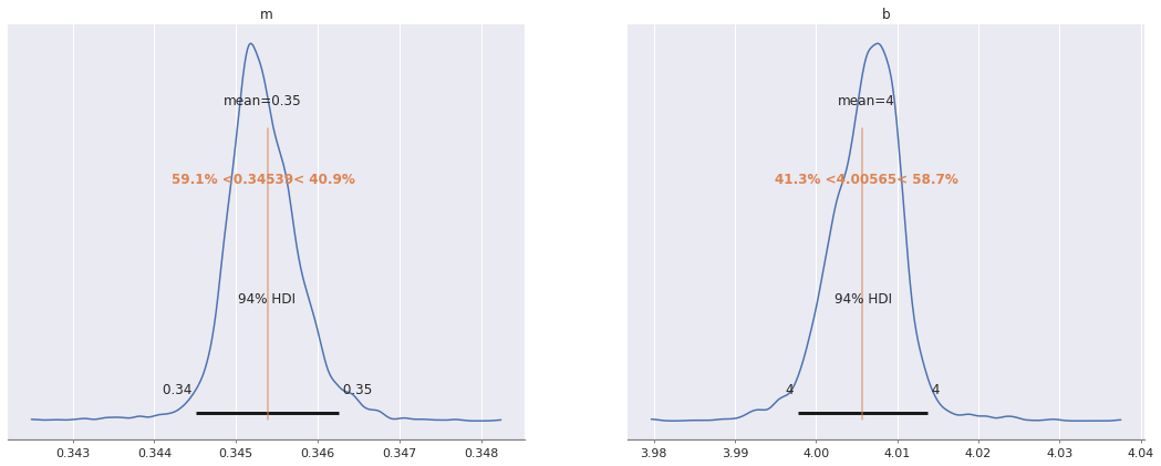
az.plot_posterior(robust_trace, var_names=["m", "b"],
                  ref_val=[m_robust, b_robust]);
fig, ax = plt.subplots()

thinned = robust_trace.posterior.stack(sample=("chain", "draw")).isel(sample=thin_slice)
ax.plot(xr_plot, xr_plot*thinned.m + thinned.b, c="C1", alpha=0.025)

ax.scatter(x, y3);

ax.axline(xy1=(0, p0), slope=p1,
          color='r', ls='--', zorder=5,
          label="NumPy OLS");

ax.axline(
    (0, ols_trace.posterior["b"].mean()),
    slope=ols_trace.posterior["m"].mean(),
    c='C0', label="PyMC OLS"
);
ax.axline(
    (0, ridge_trace.posterior["b"].mean()),
    slope=ridge_trace.posterior["m"].mean(),
    c='C1', label="PyMC Ridge"
);
ax.axline(
    (0, robust_trace.posterior["b"].mean()),
    slope=robust_trace.posterior["m"].mean(),
    c='C2', label="PyMC Robust"
);


ax.set(xlim=(-1, 15), ylim=(-2, 14));
ax.legend();
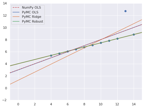
fig
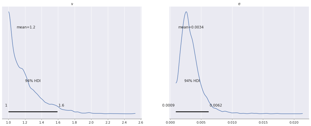
az.plot_posterior(robust_trace, var_names=["ν", "σ"]);
Hamiltonian Monte Carlo#
Bayesian inference ⇔ Differential geometry#

The Curse of Dimensionality#
def sphere_volume(d):
    return 2. * np.power(np.pi, d / 2.) / d / sp.special.gamma(d / 2)
fig, ax = plt.subplots()

d_plot = np.linspace(1, 1_000)

ax.plot(d_plot, sphere_volume(d_plot));

ax.set_xscale('log');
ax.set_xlabel("Dimensions");

ax.set_yscale('log');
ax.set_ylabel("Volume of the unit sphere");
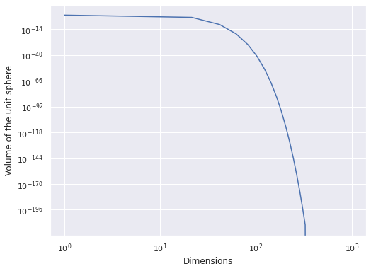
fig
Automating calculus with aesara#
x = aet.scalar("x")

y = x**3
pprint(aet.grad(y, x))
'((fill((x ** 3), 1.0) * 3) * (x ** (3 - 1)))'
A Bayesian Analysis of Lego Prices#
 |
 |
 |
Scraped from Brickset#

LEGO_DATA_URL = "https://austinrochford.com/resources/talks/data_umbrella_brickset_19800101_20211098.csv"
lego_df = pd.read_csv(LEGO_DATA_URL,
                      parse_dates=["Year released"],
                      index_col="Set number")
lego_df["Year released"] = lego_df["Year released"].dt.year
lego_df.head()
| Name | Set type | Theme | Year released | Pieces | Subtheme | RRP$ | RRP2021 | |
|---|---|---|---|---|---|---|---|---|
| Set number | ||||||||
| 1041-2 | Educational Duplo Building Set | Normal | Dacta | 1980 | 68.0 | NaN | 36.50 | 122.721632 |
| 1075-1 | LEGO People Supplementary Set | Normal | Dacta | 1980 | 304.0 | NaN | 14.50 | 48.752429 |
| 5233-1 | Bedroom | Normal | Homemaker | 1980 | 26.0 | NaN | 4.50 | 15.130064 |
| 6305-1 | Trees and Flowers | Normal | Town | 1980 | 12.0 | Accessories | 3.75 | 12.608387 |
| 6306-1 | Road Signs | Normal | Town | 1980 | 12.0 | Accessories | 2.50 | 8.405591 |
lego_df.tail()
| Name | Set type | Theme | Year released | Pieces | Subtheme | RRP$ | RRP2021 | |
|---|---|---|---|---|---|---|---|---|
| Set number | ||||||||
| 80025-1 | Sandy's Power Loader Mech | Normal | Monkie Kid | 2021 | 520.0 | Season 2 | 54.99 | 54.99 |
| 80026-1 | Pigsy's Noodle Tank | Normal | Monkie Kid | 2021 | 662.0 | Season 2 | 59.99 | 59.99 |
| 80028-1 | The Bone Demon | Normal | Monkie Kid | 2021 | 1375.0 | Season 2 | 119.99 | 119.99 |
| 80106-1 | Story of Nian | Normal | Seasonal | 2021 | 1067.0 | Chinese Traditional Festivals | 79.99 | 79.99 |
| 80107-1 | Spring Lantern Festival | Normal | Seasonal | 2021 | 1793.0 | Chinese Traditional Festivals | 119.99 | 119.99 |
lego_df.describe()
| Year released | Pieces | RRP$ | RRP2021 | |
|---|---|---|---|---|
| count | 6423.000000 | 6423.000000 | 6423.000000 | 6423.000000 |
| mean | 2009.719913 | 345.121283 | 37.652064 | 46.267159 |
| std | 8.940608 | 556.907975 | 50.917343 | 59.812083 |
| min | 1980.000000 | 11.000000 | 0.600000 | 0.971220 |
| 25% | 2003.000000 | 69.000000 | 9.990000 | 11.896044 |
| 50% | 2012.000000 | 181.000000 | 19.990000 | 27.420158 |
| 75% | 2017.000000 | 404.000000 | 49.990000 | 56.497192 |
| max | 2021.000000 | 11695.000000 | 799.990000 | 897.373477 |
VADER_MEDITATION = "75296-1"

vader_label = f"{lego_df.loc[VADER_MEDITATION, 'Name']} ({VADER_MEDITATION.split('-')[0]})"
ax = sns.scatterplot(x="Pieces", y="RRP2021", data=lego_df,
                     alpha=0.5)
ax.scatter(lego_df.loc[VADER_MEDITATION, "Pieces"],
           lego_df.loc[VADER_MEDITATION, "RRP2021"],
           c='r', label=vader_label);

ax.set_xscale('log');

ax.set_yscale('log');
ax.set_ylabel("Recommended retail price\n(2021 $)");

ax.legend();
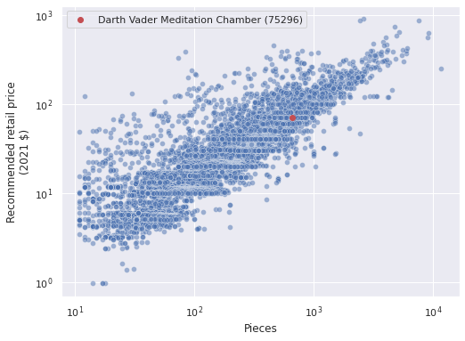
ax.figure
lego_df["PPP2021"] = lego_df["RRP2021"] / lego_df["Pieces"]
ax = sns.stripplot(x="Year released", y="PPP2021", data=lego_df,
                   jitter=0.25, color='C0', alpha=0.5)
ax.scatter(lego_df.loc[VADER_MEDITATION, "Year released"] - lego_df["Year released"].min(),
           lego_df.loc[VADER_MEDITATION, "PPP2021"],
           c='r', zorder=10, label=vader_label);

ax.xaxis.set_major_locator(ticker.MultipleLocator(5));

ax.set_yscale('log');
ax.set_ylabel("Recommended retail price\nper piece (2021 $)");

ax.legend();
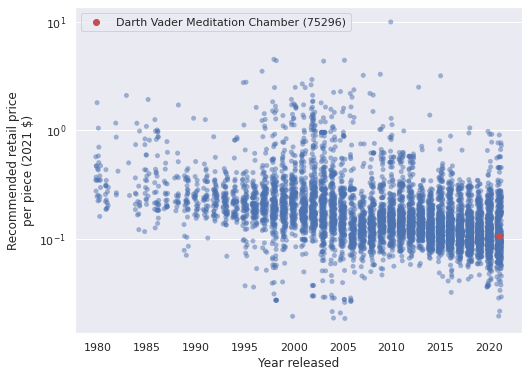
ax.figure
PLOT_THEMES = ["Star Wars", "Creator", "Disney", "Harry Potter"]
ax = sns.stripplot(
    x="Year released", y="PPP2021", hue="Theme",
    data=lego_df.assign(
       Theme=lego_df["Theme"]
                    .where(lego_df["Theme"].isin(PLOT_THEMES),
                           "Other")
   ),
   jitter=0.25, dodge=True, alpha=0.5
)

ax.xaxis.set_major_locator(ticker.MultipleLocator(5));

ax.set_yscale('log');
ax.set_ylabel("Recommended retail price\nper piece (2021 $)");

ax.legend(loc='upper left');
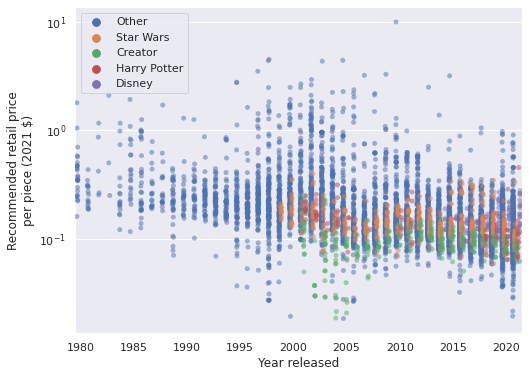
ax.figure
Price model#
log_pieces = (lego_df["Pieces"]
                     .pipe(np.log)
                     .values)

scaler = StandardScaler().fit(log_pieces[:, np.newaxis])

def scale_log_pieces(log_pieces, scaler=scaler):
    return scaler.transform(log_pieces[:, np.newaxis])[:, 0]

std_log_pieces = scale_log_pieces(log_pieces)
log_rrp2021 = (lego_df["RRP2021"]
                      .pipe(np.log)
                      .values)
theme_id, theme_map = lego_df["Theme"].factorize(sort=True)
year = lego_df["Year released"].values
t = year - year.min()
def noncentered_normal(name, *, dims, μ=None):
    μ = pm.Normal(f"μ_{name}", 0., 2.5)
    Δ = pm.Normal(f"Δ_{name}", 0., 1., dims=dims)
    σ = pm.HalfNormal(f"σ_{name}", 2.5)

    return pm.Deterministic(name, μ + Δ * σ, dims=dims)

def gaussian_random_walk(name, *, dims, innov_scale=1.):
    Δ = pm.Normal(f"Δ_{name}", 0., innov_scale,  dims=dims)

    return pm.Deterministic(name, Δ.cumsum(), dims=dims)
coords = {
    "set": lego_df.index,
    "theme": theme_map,
    "year": np.unique(year)
}
with pm.Model(coords=coords) as lego_model:
    β0_t = gaussian_random_walk("β0_t", dims="year", innov_scale=0.1)
    β0_theme = noncentered_normal("β0_theme", dims="theme")

    β_piece_t = gaussian_random_walk("β_piece_t", dims="year", innov_scale=0.1)
    β_piece_theme = noncentered_normal("β_piece_theme", dims="theme")

    σ = pm.HalfNormal("σ", 5.)
    μ = β0_t[t] + β0_theme[theme_id] \
        + (β_piece_t[t] + β_piece_theme[theme_id]) * std_log_pieces \
        - 0.5 * σ**2

    obs = pm.Normal("obs", μ, σ, dims="set", observed=log_rrp2021)
Why Hamiltonian Monte Carlo?#
CHAINS = 3

SAMPLE_KWARGS = {
    'cores': CHAINS,
    'random_seed': [SEED + i for i in range(CHAINS)]
}
with lego_model:
    mh_lego_trace = pm.sample(draws=10_000, step=pm.Metropolis(),
                              **SAMPLE_KWARGS)
/home/oriol/miniconda3/envs/arviz/lib/python3.9/site-packages/pymc/model.py:984: FutureWarning: `Model.initial_point` has been deprecated. Use `Model.recompute_initial_point(seed=None)`.
  warnings.warn(
/home/oriol/miniconda3/envs/arviz/lib/python3.9/site-packages/pymc/model.py:984: FutureWarning: `Model.initial_point` has been deprecated. Use `Model.recompute_initial_point(seed=None)`.
  warnings.warn(
/home/oriol/miniconda3/envs/arviz/lib/python3.9/site-packages/pymc/model.py:984: FutureWarning: `Model.initial_point` has been deprecated. Use `Model.recompute_initial_point(seed=None)`.
  warnings.warn(
/home/oriol/miniconda3/envs/arviz/lib/python3.9/site-packages/pymc/model.py:984: FutureWarning: `Model.initial_point` has been deprecated. Use `Model.recompute_initial_point(seed=None)`.
  warnings.warn(
/home/oriol/miniconda3/envs/arviz/lib/python3.9/site-packages/pymc/model.py:984: FutureWarning: `Model.initial_point` has been deprecated. Use `Model.recompute_initial_point(seed=None)`.
  warnings.warn(
Multiprocess sampling (3 chains in 3 jobs)
/home/oriol/miniconda3/envs/arviz/lib/python3.9/site-packages/pymc/model.py:984: FutureWarning: `Model.initial_point` has been deprecated. Use `Model.recompute_initial_point(seed=None)`.
  warnings.warn(
Sampling 3 chains for 1_000 tune and 10_000 draw iterations (3_000 + 30_000 draws total) took 61 seconds.
The rhat statistic is larger than 1.4 for some parameters. The sampler did not converge.
The estimated number of effective samples is smaller than 200 for some parameters.
mh_lego_rhat = az.rhat(mh_lego_trace)
fig, ax = plt.subplots()

max_rhat = (mh_lego_rhat.max()
                        .to_array())
nvar, = max_rhat.shape

ax.barh(np.arange(nvar), max_rhat);
ax.axvline(1, c='k', ls='--', label="Convergence");

ax.set_xlim(left=0.8);
ax.set_xlabel(r"$\hat{R}$");

ax.set_yticks(np.arange(nvar));
ax.set_yticklabels(max_rhat.coords["variable"].to_numpy()[::-1]);

ax.legend();
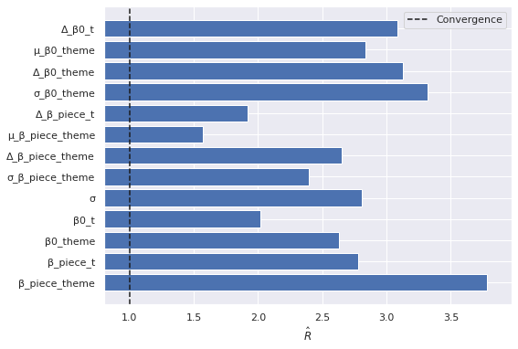
fig
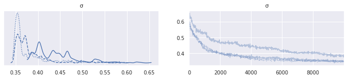
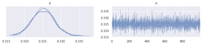
az.plot_trace(mh_lego_trace, var_names="σ");
This model has
n_lego_param = sum([
    coords["year"].size,  # time intercept increments
    coords["theme"].size, # theme intercept offsets
    2,                    # theme intercept location and scale
    coords["year"].size,  # time slope increments
    coords["theme"].size, # theme slope offsets
    2,                    # theme intercept location and scale
    1                     # scale of observational noise
])
n_lego_param
351
parameters
fig, ax = plt.subplots()

d_plot = np.linspace(1, 1_000)

ax.plot(d_plot, sphere_volume(d_plot));
ax.axvline(n_lego_param, c='k', ls='--', label=f"{n_lego_param} dimensions");

ax.set_xscale('log');
ax.set_xlabel("Dimensions");

ax.set_yscale('log');
ax.set_ylabel("Volume of the unit sphere");

ax.legend();
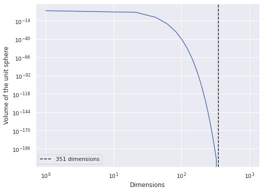
fig
with lego_model:
    lego_trace = pm.sample(**SAMPLE_KWARGS)
    lego_trace.extend(pm.sample_posterior_predictive(lego_trace))
Auto-assigning NUTS sampler...
Initializing NUTS using jitter+adapt_diag...
/home/oriol/miniconda3/envs/arviz/lib/python3.9/site-packages/pymc/model.py:984: FutureWarning: `Model.initial_point` has been deprecated. Use `Model.recompute_initial_point(seed=None)`.
  warnings.warn(
Multiprocess sampling (3 chains in 3 jobs)
NUTS: [Δ_β0_t, μ_β0_theme, Δ_β0_theme, σ_β0_theme, Δ_β_piece_t, μ_β_piece_theme, Δ_β_piece_theme, σ_β_piece_theme, σ]
Sampling 3 chains for 1_000 tune and 1_000 draw iterations (3_000 + 3_000 draws total) took 509 seconds.
The number of effective samples is smaller than 10% for some parameters.
/home/oriol/miniconda3/envs/arviz/lib/python3.9/site-packages/pymc/backends/arviz.py:380: UserWarning: The shape of variables  in posterior_predictive group is not compatible with number of chains and draws. The automatic dimension naming might not have worked. This can also mean that some draws or even whole chains are not represented.
  warnings.warn(
lego_rhat = az.rhat(lego_trace).max()
fig, ax = plt.subplots()

max_rhat = (lego_rhat.max()
                     .to_array())
nvar, = max_rhat.shape

ax.barh(np.arange(nvar), max_rhat);
ax.axvline(1, c='k', ls='--', label="Convergence");

ax.set_xlim(left=0.95);
ax.set_xlabel(r"$\hat{R}$");

ax.set_yticks(np.arange(nvar));
ax.set_yticklabels(max_rhat.coords["variable"].to_numpy()[::-1]);

ax.legend();
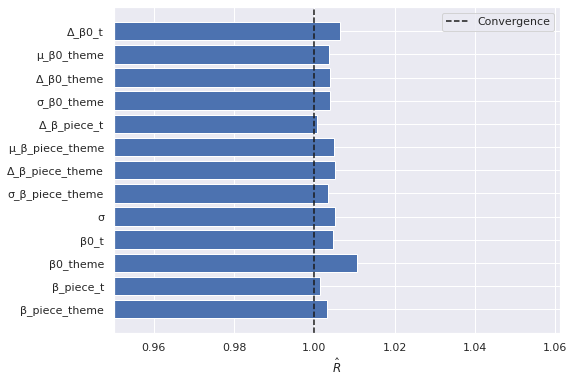
fig
az.plot_trace(mh_lego_trace, var_names="σ");
az.plot_trace(lego_trace, var_names="σ");
sampling_time = np.array([
    mh_lego_trace.sample_stats.sampling_time,
    lego_trace.sample_stats.sampling_time
])

σ_ess = np.array([
    az.ess(mh_lego_trace, var_names="σ")["σ"],
    az.ess(lego_trace, var_names="σ")["σ"]
])

σ_esps = σ_ess / sampling_time
fig, axes = plt.subplots(ncols=2, sharex=True,
                         figsize=(2 * FIG_WIDTH, FIG_HEIGHT))

axes[0].bar([0, 1], sampling_time);

axes[0].set_xticks([0, 1]);
axes[0].set_xticklabels(["Metropolis-Hastings", "Adaptive HMC (NUTS)"]);

axes[0].set_yscale('log');
axes[0].set_ylabel("Sampling time");

axes[1].bar([0, 1], σ_esps);

axes[1].set_ylabel("Effective samples per second");

fig.suptitle("Sampling efficiency");
fig.tight_layout();
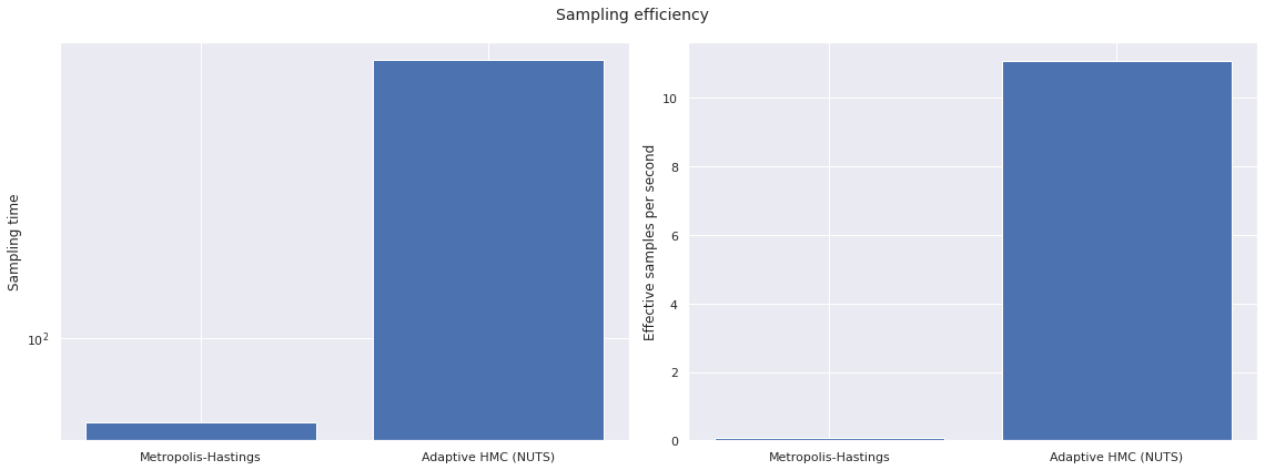
fig
To get the same effective sample size as adaptive HMC (NUTS) with Metropolis-Hastings would required approximately
σ_ess[1] / σ_esps[0] / 60 / 60
22.963846852430844
hours.
def format_posterior_artist(artist, formatter):
    text = artist.get_text()
    x, _ = artist.get_position()

    if text.startswith(" ") or text.endswith(" "):
        fmtd_text = formatter(x)
        artist.set_text(
            " " + fmtd_text if text.startswith(" ") else fmtd_text + " "
        )
    elif "=" in text:
        before, _ = text.split("=")
        artist.set_text("=".join((before, formatter(x))))
    elif "<" in text:
        below, ref_val_str, above = text.split("<")
        artist.set_text("<".join((
            below,
            " " + formatter(float(ref_val_str)) + " ",
            above
        )))

def format_posterior_text(formatter, ax=None):
    if ax is None:
        ax = plt.gca()

    artists = [artist for artist in ax.get_children() if isinstance(artist, plt.Text)]

    for artist in artists:
        format_posterior_artist(artist, formatter)
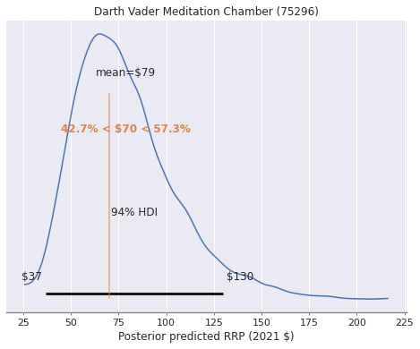
Is Darth Vader’s Meditation Chamber priced fairly?#
%%capture
ax = az.plot_posterior(
    lego_trace, group="posterior_predictive",
    coords={"set": VADER_MEDITATION},
    transform=np.exp, ref_val=lego_df.loc[VADER_MEDITATION, "RRP2021"]
)
format_posterior_text(dollar_formatter, ax=ax);

ax.set_xlabel("Posterior predicted RRP (2021 $)");
ax.set_title(vader_label);
ax.figure
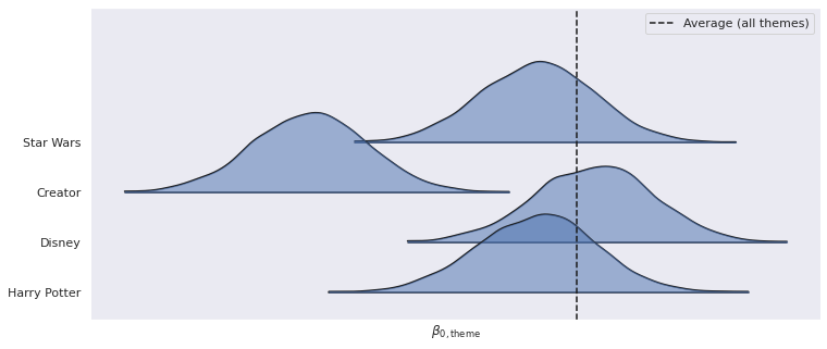
%%capture
ax, = az.plot_forest(
    lego_trace, var_names="β0_theme",
    coords={"theme": PLOT_THEMES}, combined=True,
    kind='ridgeplot', ridgeplot_alpha=0.5,
    ridgeplot_truncate=False, hdi_prob=1
)

ax.axvline(lego_trace.posterior["μ_β0_theme"]
                     .mean(dim=("chain", "draw")),
           c='k', ls='--', label="Average (all themes)");
ax.set_xticks([]);
ax.set_xlabel(r"$\beta_{0, \mathrm{theme}}$");

ax.set_yticklabels(PLOT_THEMES[::-1]);

ax.legend();
ax.figure
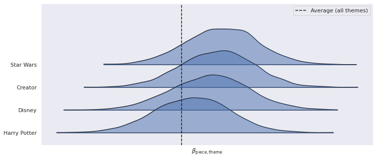
%%capture
ax, = az.plot_forest(
    lego_trace, var_names="β_piece_theme",
    coords={"theme": PLOT_THEMES}, combined=True,
    kind='ridgeplot', ridgeplot_alpha=0.5,
    ridgeplot_truncate=False, hdi_prob=1
)

ax.axvline(lego_trace.posterior["μ_β_piece_theme"]
                     .mean(dim=("chain", "draw")),
           c='k', ls='--', label="Average (all themes)");
ax.set_xticks([]);
ax.set_xlabel(r"$\beta_{\mathrm{piece}, \mathrm{theme}}$");

ax.set_yticklabels(PLOT_THEMES[::-1]);

ax.legend();
ax.figure
Next steps#
 |
 |
Thank you!#